


Consistent hashing for even load distribution
Table of contents
Document Engine is a Nutrient platform designed to provide a complete SDK for managing the full lifecycle of a document — from storing or generating a document, through viewing and editing, to exporting from the system.
It’s a solution for managing massive amounts of documents while providing concurrent access for thousands of users. This, however, raises a fundamental challenge Document Engine needs to address: How can we effectively provide access to all resources?
Document storage and the caching challenge
An ordinary block storage-based file system isn’t suitable for storing documents. When uploading a document to Document Engine, the file is stored either directly in a Postgres database or in one of the configured asset storages. We currently support AWS S3 (and compatible services) and Azure Blob Storage.
This provides good storage capabilities; however, it doesn’t enable us to handle documents directly.
On every access to a document, it needs to be downloaded from asset storage. Only after that can it be loaded fully or partially into memory — for example, for rendering. In this scenario, the time to access a document is largely limited by two factors: transfer bandwidth and document size.
A simple mitigation for this problem is a file system cache that keeps the document on the local file system after it has been downloaded. That’s where Document Engine comes in.
Document Engine uses a least recently used (LRU) cache, which keeps documents on the local file system while keeping the total cache size within a configurable limit. When the limit is reached, the least recently accessed cached documents are removed.
This effectively enables data locality, meaning documents that are accessed more often are kept in the cache and don’t need to be downloaded from asset storage.
The scaling problem: When caching breaks down
This solution is efficient at low scale, but as the number of documents and users accessing them increases, it approaches the limits of this performance optimization.
While this issue isn’t as noticeable for small documents that can be quickly downloaded and cached, it becomes a significant problem for large documents, where download times can reach several seconds or even minutes. When the system stores tens of terabytes and the access pattern to documents is uniform, the cache hit rate drops dramatically. Large documents are frequently evicted from the cache before they can be reused, forcing repeated downloads from asset storage and severely impacting user experience.
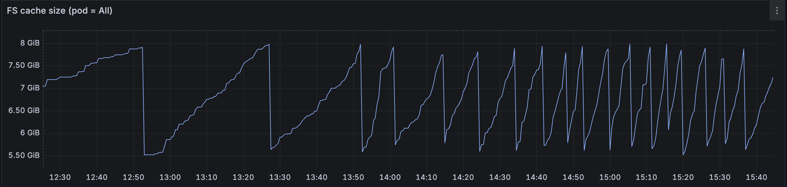
The figure above shows the cache size for a Document Engine installation with an 8GB cache configured. The cache grows constantly and periodically gets reduced when the LRU algorithm triggers, clearing 30 percent of the cached storage space by removing the least recently used documents. This pattern suggests that the miss rate is very high and files need to be downloaded from asset storage frequently.
Adding more nodes to the cluster won’t help with performance, as requests aren’t routed by document IDs but are instead uniformly distributed across the cluster. This means that different nodes are handling the same documents, which results in the cache being duplicated across nodes. Each node maintains its own separate cache, so popular documents end up being stored multiple times across different nodes, wasting precious cache space.
Moreover, when a user requests a document that was previously cached on a different node, it still needs to be downloaded from asset storage, defeating the purpose of caching. This leads to poor cache utilization and increased network traffic to asset storage.
How can data locality be ensured in such an environment?
Enter consistent hashing
The naive solution would be to increase the cache size. Unfortunately, this isn’t always possible, and it raises the question: How much cache is enough? Besides, the cache size needs to be increased across all nodes, which means ephemeral storage consumption is multiplied by the number of nodes in the cluster.
The solution to this problem is to use the consistent hashing algorithm. Consistent hashing is a technique that allows you to distribute the load evenly across multiple nodes. It’s used in many distributed systems, such as caches, databases, and file systems. The idea is to use a hash function to map documents to shards. This way, documents are evenly distributed across the shards, the load is balanced, and duplication is mitigated.
First, we need to define the shards. Document Engine is designed to run in a cluster, which means multiple instances of Document Engine can run at the same time. A shard represents the part of the hash value space that should be assigned to a given Document Engine node. The instances of Document Engine are identified by their unique IDs, which are used to place them in the hash value space. It’s as simple as hashing the node’s ID.
For each document, we need to calculate the hash value using the consistent hashing algorithm. The hash value is then used to determine which shard the document belongs to by finding the “next” value in the hash value space belonging to a Document Engine instance.
But what if there’s no “next” shard? Which shard should the document be assigned to? In this case, the algorithm wraps around to the beginning of the hash space and selects the first shard (represented by the node with the smallest hash value).
This wraparound behavior is what makes the hash space “circular.” As shown in the diagram below, the hash space goes from 0 to some maximum (4,294,967,295 (2^32) in the diagram) and then wraps back to 0. That’s why the hash space is commonly referred to as a “hash ring.”
This ensures that every document is always assigned to exactly one node, regardless of its hash value.
Hash ring
   Hash space: 0 ────────────────────────────────────── 4,294,967,295 (2^32)                                    (wraps around)
              0                      2,147,483,648               4,294,967,295              |                            |                            |              ▼                            ▼                            ▼         ┌─────────────────────────────────────────────────────────────────┐         │         A                      B                      C         │         │         │                      │                      │         │         └─────────┼──────────────────────┼──────────────────────┼─────────┘                   │                      │                      │                Node A                 Node B                 Node C           (hash: 500M)            (hash: 2.1B)           (hash: 3.8B)
When we want to store a document, after assigning it a unique ID, we can calculate the hash value of the ID and find the closest node in the hash ring:
Document: "document.pdf" ┌───────────┐ │ hash(key) │ ──► Hash: 1,500,000,000 └───────────┘ │ ▼ ┌───────────────────────────────────────────┐ │ Find first shard ≥ 1,500,000,000 in ring │ └───────────────────────────────────────────┘ │ ▼ Ring position: 2,147,483,648 │ ▼ ┌─────────────┐ │ Node B │ ◄── Document handled by this node └─────────────┘The new document hash is 1,500,000,000, so we find the corresponding shard in the hash ring. The next shard is Node B, which has a hash value of 2,147,483,648.
Let’s look at a different example. Say we have a document with a hash value of 4,000,000,000. Since all our nodes (A: 500M, B: 2.1B, C: 3.8B) have smaller hash values, there’s no next shard. In this case, the algorithm wraps around to the beginning of the ring and assigns the document to Node A (the first node, with hash value 500M). This wraparound behavior ensures every document always gets assigned to a node.
Now, when we want to access a document, we can calculate the hash value of the document ID, and by knowing the cluster topology, we can find the node responsible for the document without needing to access the node or even query the cluster.
How to shoot ourselves in the foot
Still, this solution has a problem with load distribution. The node names are randomly distributed across the hash space, which means some nodes may have more documents than others. In an extreme case, one node may have all the documents, while the others have none:
   Hash space: 0 ────────────────────────────────────── 4,294,967,295 (2^32)                                    (wraps around)
              0                      2,147,483,648               4,294,967,295              |                            |                            |              ▼                            ▼                            ▼         ┌─────────────────────────────────────────────────────────────────┐         │         A  B  C                                                 │         │         │  │  │                                                 │         └─────────┼──┼──┼─────────────────────────────────────────────────┘                   │  │  └───────────────────────────────────────┐                   │  └──────────────────┐                       │                Node A                 Node B                 Node C           (hash: 500M)            (hash: 501M)           (hash: 502M)
In this case, the load isn’t evenly distributed across the nodes, which means some nodes may be overloaded while others are idle.
Hash ranges: ┌─────────────────┬────────────────────┬─────────────────────────────────┐ │ Range │ Assigned to node │ Percentage of hash space │ ├─────────────────┼────────────────────┼─────────────────────────────────┤ │ 0 → 500M │ Node A │ 11.6% (500M/4.3B) │ ← OVERLOADED │ 500M → 501M │ Node B │ 0.2% (1M /4.3B) │ │ 501M → 502M │ Node C │ 0.2% (1M /4.3B) │ │ 502M → 4.3B │ Node A (wraparound)│ 88.3% (500M/4.3B) │ ← OVERLOADED └─────────────────┴────────────────────┴─────────────────────────────────┘As a result, we’ll practically handle all the documents on Node A, while nodes B and C will be idle.
Solution: Virtual sharding
To solve this problem, we can assign more shards to each node. With this approach, it’s almost impossible to have a situation where one node has all the documents.
Instead of hashing the node IDs directly, we can hash the ID together with an integer — like {node_id, 0}, {node_id, 1}, {node_id, 2}, etc. — up to a configured limit. This way, we can create multiple virtual shards for each actual node, which will be evenly distributed across the hash space.
Here’s the hash ring structure (simplified — showing fewer shards than in reality):
   Hash Space: 0 ────────────────────────────────────── 4,294,967,295 (2^32)                                    (wraps around)
              0        1073741824      2147483648      3221225472              |            |              |              |              ▼            ▼              ▼              ▼         ┌────────────────────────────────────────────────────────┐         │    A1    B2    A3    C1    B4    A5    C3    B6        │         │     │     │     │     │     │     │     │     │        │         └─────┼─────┼─────┼─────┼─────┼─────┼─────┼─────┼────────┘               │     │     │     │     │     │     │     │            Node A Node B Node A Node C Node B Node A Node C Node B
   A1, A3, A5 = Node A’s virtual shards (hash({node_a, 1}), etc.)   B2, B4, B6 = Node B’s virtual shards   C1, C3     = Node C’s virtual shards
Advantages of consistent hashing
Why is this approach better than just using a simple hash function? It would also distribute the documents across the nodes, right?
The main advantage of consistent hashing is that it allows you to add or remove nodes from the cluster without having to move all the documents.
With simple hashing:
my_node = hash(document_id) % number_of_nodes
Changing the number of nodes would require reassigning all the documents to the new nodes.
The algorithm guarantees that when a new node is added to the cluster, only a small number of documents will be moved to the new node.
Also, when a node is removed from the cluster, only a small number of documents will be moved to the remaining nodes, and they’ll be distributed evenly across the remaining nodes.
Let’s consider an example of node removal.
┌─────────────┐ ┌─────────────┐ ┌─────────────┐ │ Node A │ │ Node B │ │ Node C │ │ │ │ │ │ │ │ Documents: │ │ Documents: │ │ Documents: │ │ • doc_001 │ │ • doc_004 │ │ • doc_007 │ │ (shard A1) │ │ (shard B1) │ │ (shard C1) │ │ │ │ │ │ │ │ • doc_002 │ │ • doc_005 │ │ • doc_008 │ │ (shard A2) │ │ (shard B2) │ │ (shard C3) │ │ │ │ │ │ │ │ • doc_003 │ │ • doc_006 │ │ • doc_009 │ │ (shard A3) │ │ (shard B3) │ │ (shard C3) │ │ │ │ │ │ │ └──────┬──────┘ └──────┬──────┘ └──────┬──────┘ │ │ │ └──────────────────┼──────────────────┘ │ ┌────────┴────────┐ │ Load balancer │ │ │ │ Routes based on │ │ consistent hash │ └─────────────────┘The hash space looks like this: [A1] - [B1] - [A2] - [C1] - [B2] - [A3] - [C2] - [B3] - [C3]
When we remove Node B, the documents that were assigned to Node B will be moved to the remaining nodes, Node A and Node C.
Hash space after Node B removal: [A1] - [B1] - [A2] - [C1] - [B2] - [A3] - [C2] - [B3] - [C3]
The documents will be moved to the remaining nodes, A and C.
┌─────────────┐ ┌─────────────┐ │ Node A │ │ Node C │ │ │ │ │ │ Documents: │ │ Documents: │ │ • doc_001 │ │ • doc_007 │ │ (shard A1) │ │ (shard C1) │ │ │ │ │ │ • doc_002 │ │ • doc_008 │ │ (shard A2) │ │ (shard C3) │ │ │ │ │ │ • doc_003 │ │ • doc_009 │ │ (shard A3) │ │ (shard C3) │ │ │ │ │ │ + doc_004 │ │ + doc_006 │ │ (shard A2) │ │ (shard C3) │ │ │ │ │ │ + doc_005 │ │ │ │ (shard A3) │ │ │ │ │ │ │ └──────┬──────┘ └───────┬─────┘ │ │ └───────────┬───────────┘ │ │ ┌─────────┴───────┐ │ Load balancer │ │ │ │ Routes based on │ │ consistent hash │ └─────────────────┘Conclusion
Document Engine faced performance challenges due to file system cache limitations when handling large document collections. By implementing consistent hashing with virtual shards, we created a distributed caching system that:
- Distributes documents evenly across multiple nodes
- Minimizes data movement during cluster topology changes
- Provides deterministic document-to-node mapping
- Maintains high availability during node failures
This solution scales Document Engine’s caching capabilities horizontally while maintaining the simplicity of the original LRU cache design at each individual node.
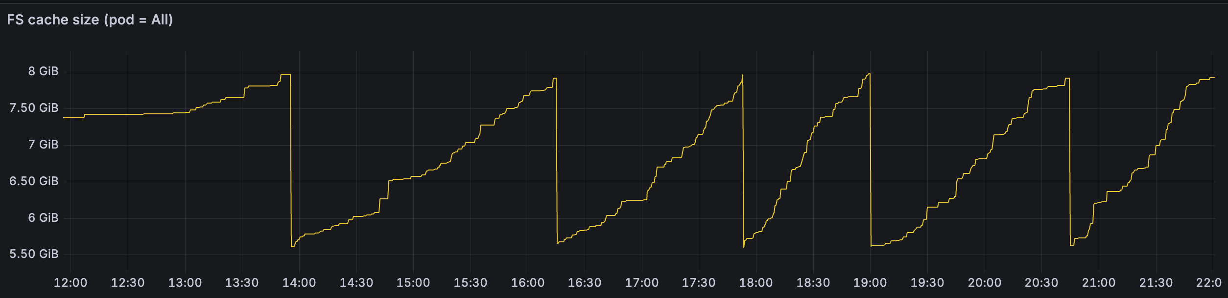
The graph above shows the cache size dynamics for the same Document Engine installation, but with consistent hashing enabled. Notice that with the same number of nodes and identical workload, the LRU cache cleanup now occurs approximately once every 1–2 hours, compared to roughly every 5 minutes in the previous implementation. Also note that this graph spans 10 hours, compared to the 5-hour timeframe shown in the earlier graph, further highlighting the dramatic improvement in cache efficiency.